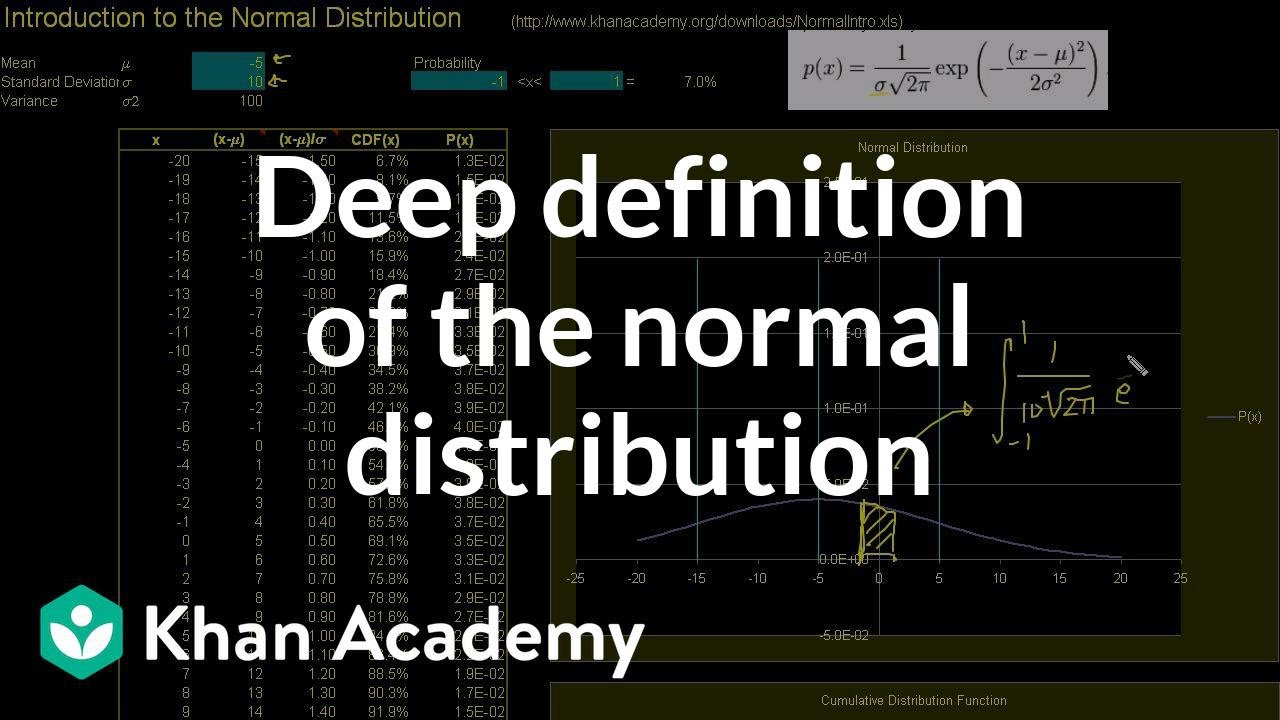
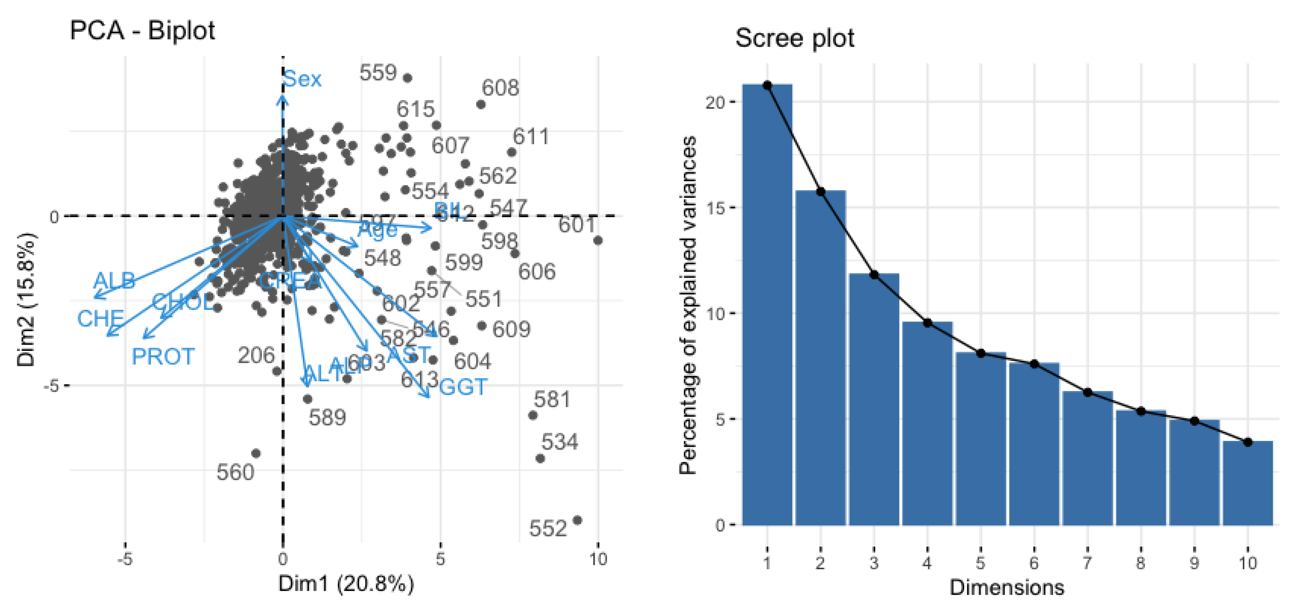
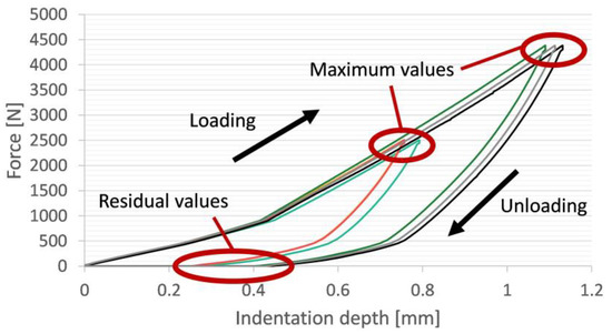
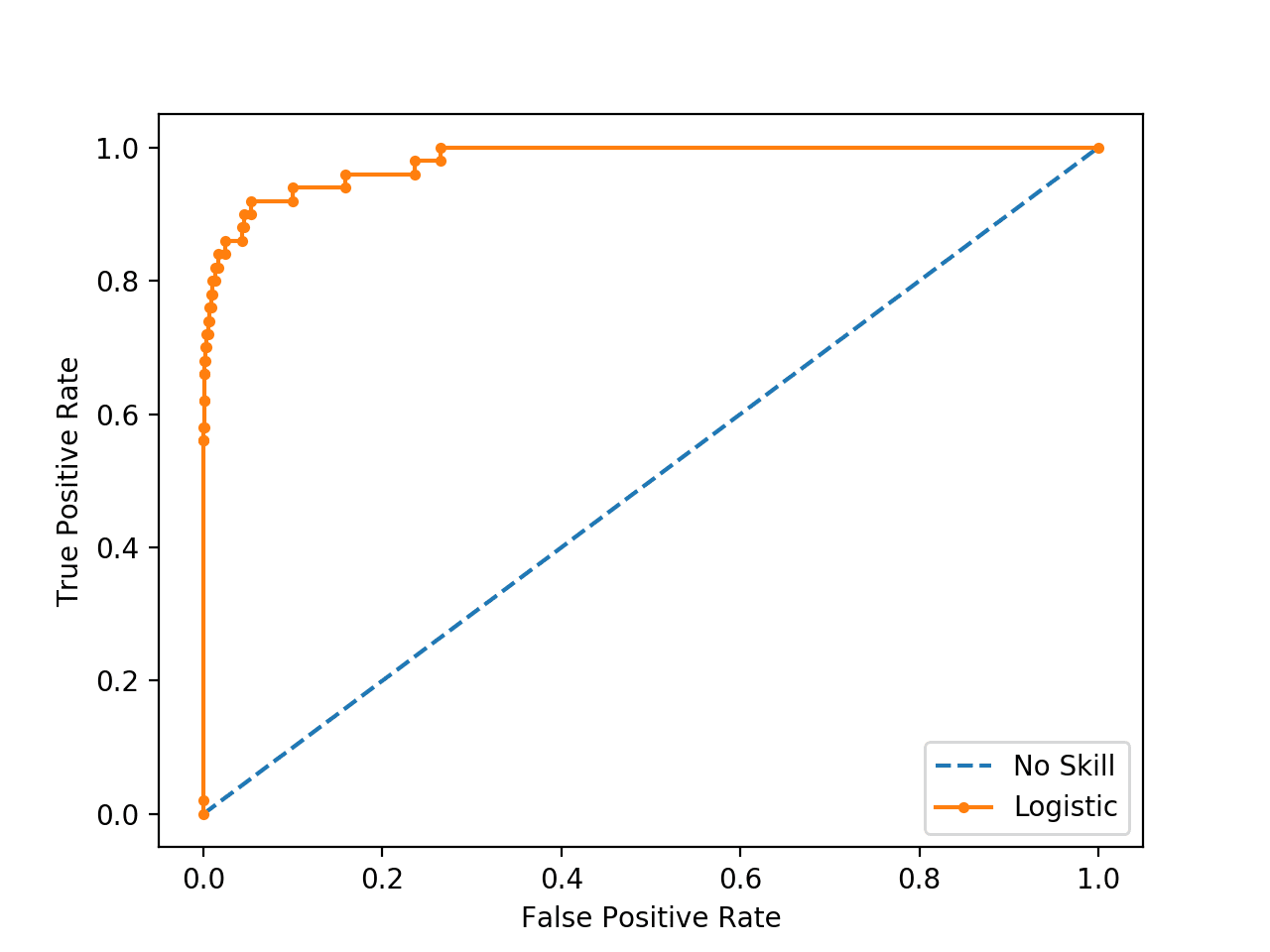
39 refer to the diagram to the right. curve g approaches curve f because

D. aggregate supply has increased and the price level has risen to G. 35. Refer to the above diagram. If aggregate supply is AS1 and aggregate demand is AD0, then: A. at any price level above G a shortage of real output would occur. B. F represents a price level that would result in a surplus of real output of AC. Refer to the diagram to the right which shows the demand and supply curves for the almond market. The government believes that the equilibrium price is too low and tries to help almond growers by setting a price floor at Pf. ... Refer to the diagram to the right. Curve G approaches curve F because. average fixed costs falls as output rises ...

Refer to the curve shown below. plane from an airport during a long flight. ... The composition g f involves arranging the machines so the original input goes into f , and the output from f then becomes the input for g (see right side of margin figure). √ Example 2. ... (see margin). If we let x approach 3 from the right (x is close to 3 and ...

Refer to the diagram to the right. curve g approaches curve f because

for the ARMA model that makes it easy for you to derive the state equations.) Remark: multi-input, multi-output time-series models (i.e., u(k) ∈ Rm, y(k) ∈ Rp) are readily handled by allowing the coefficients ai, bi to be matrices. 2.4 Representing linear functions as matrix multiplication. Curve G approaches curve F because - ScieMce. Refer to Figure 11-5. Curve G approaches curve F because. A) marginal cost is above average variable costs. B) fixed cost falls as capacity rises. C) average fixed cost falls as output rises. D) total cost falls as more and more is produced. Refer to Figure 11-5. Curve G approaches curve F because a)total cost falls as more and more is produced. b)marginal cost is above average variable costs c)fixed cost falls as capacity rises. d)average fixed cost falls as output rises.

Refer to the diagram to the right. curve g approaches curve f because. Benchmark Dose Approach (2) 1. A mathematical model is applied to the experimental data to produce a dose-response curve of best fit. 2. By statistical calculation an upper 95% confidence limit of the curve is determined 3. The Benchmark Response is defined as 10% (or 5%, or 1%). 4. The Benchmark Dose corresponds to the bench indifference curves cross BL2, IC2 through point B represents the highest utility level given BL2. (IC2 is the pink linear indifference curve in our graph). The economic meaning is also obvious, since coffee and tea are perfect substitutes for Lisa and the price of coffee is cheaper than the price of tea, she would only consume coffee now! Refer to the diagram to the right the vertical difference between curves f and g measures. B intersects the horizontal axis at a point corresponding to the 5th worker. In a diagram that shows the marginal product of labor on the vertical axis and labor on the horizontal axis the marginal product curve 10 a never intersects the horizontal axis. Shift curve a to the left and shift curve b downward. Refer to the diagram to the right curve g approaches curve f because. A firm finds that at its mrmc output its tc 1000 tvc 800 tfc 200 and total revenue is 900. Curve g approaches curve f because a fixed cost falls as capacity rises.

Refer to the diagram to the right. Curve G approaches curve F because. average fixed costs falls as output rises. ... Refer to the diagram to the right which shows short run cost and demand curves for a monopolistically competitive firm in the market for designer watches. 24. Curve G approaches curve F because - marginal cost is above average variable costs. - fixed cost falls as capacity rises. - total cost falls as more and more is produced. - average fixed cost falls as output rises. Refer to the diagram to the right. Curve G approaches curve F because A. average fixed costs falls as output rises. B. fixed costs falls as capacity rises. C. total costs fall as more and more is produced. D. marginal costs are above average variable costs. Derivation of the IS Curve: The equilibrium condition in the goods market in terms of income expenditure approach is. Y = C + I + G …. (5) ADVERTISEMENTS: In terms of the leakage-injection approach the condition is. I + G = S + T …. (6) If we ignore the government sector (i.e., if G and T are zero), we can express equation (6) as.

A. rightward shift in the economy's aggregate demand curve. B. rightward shift in the economy's aggregate supply curve. C. movement along an existing aggregate demand curve. D. leftward shift in the economy's aggregate demand curve. 6. If the MPS in an economy is .1, government could shift the aggregate demand curve rightward by $40 billion by: the IS curve steeper. d) Movement south-east along the IS curve. e) IS curve flatter. f) .This is equivalent to a higher MPC in the consumption function. It has the same effect, i.e. increases the size of the multiplier, making the IS curve flatter. 7. Imagine you are running a safe house in the early 19th century. Assume there are D) E = marginal cost curve; F = total cost curve; G = variable cost curve, H = average fixed cost curve. 33) Refer to Figure 10-4. The vertical difference between curves F and G measures. A) average fixed costs. B) sunk costs. C) marginal costs. D) fixed costs. 34) Refer to Figure 10-4. Curve G approaches curve F because. A) fixed costs falls ... C. concave to the origin because of increasing opportunity costs. D. convex to the origin because of increasing opportunity costs. 6. If all discrimination in the United States were eliminated, the economy would: A. have a less concave production possibilities curve. B. produce at some point closer to its production possibilities curve.

a. supply curve upward (or to the left). b. supply curve downward (or to the right). c. demand curve upward (or to the right). d. demand curve downward (or to the left). ____ 25. When a tax is imposed on a good for which demand is elastic and supply is elastic, a. sellers effectively pay the majority of the tax.

Q: Refer to the diagram to the right. Curve G approaches curve F because A: average fixed costs falls as output rises. Q: Refer to the diagram to the right. Diminishing marginal productivity sets in after A: the 2nd worker is hired.

G. Thus, the IS curve is vertical at this level, as shown in the Figure. Monetary policy has no effect on output, because the IS curve determines Y. Monetary policy can affect only the interest rate. In contrast, fiscal policy is effective: output increases by the full amount that the IS curve shifts.

average fixed cost curve. 21) Refer to Figure 11 -5. The vertical difference between curves F and G measures 21) A) marginal costs. B) fixed costs. C) average fixed costs. D) sunk costs. 22) Refer to Figure 11 -5. Curve G approaches curve F because 22) A) fixed cost falls as capacity rises. B) total cost falls as more and more is produced.

Economics. Economics questions and answers. Curve G approaches curve F because marginal cost is above average variable costs. average fixed cost falls as output rises. Identify the curves in the diagram. E = average fixed cost curve; F = variable cost curve; G = total cost curve, H = marginal cost curve E = marginal cost curve; F = total cost ...

Phase diagram is a graphical representation of the physical states of a substance under different conditions of temperature and pressure. A typical phase diagram has pressure on the y-axis and temperature on the x-axis. As we cross the lines or curves on the phase diagram, a phase change occurs. In addition, two states of the substance coexist ...

Consider the phase diagram for carbon dioxide shown in Figure 5 as another example. The solid-liquid curve exhibits a positive slope, indicating that the melting point for CO 2 increases with pressure as it does for most substances (water being a notable exception as described previously). Notice that the triple point is well above 1 atm, indicating that carbon dioxide cannot exist as a liquid ...

shift the LM curve at all. 2) Use the IS-LM diagram to describe the short-run and long-run effects of the following changes on national income, the interest rate, the price level, consumption, investment, and real money balances. a) An increase in the money supply. An increase in the money supply shifts the LM curve to the right in the short run.

Refer to Figure 11-5. Curve G approaches curve F because a)total cost falls as more and more is produced. b)marginal cost is above average variable costs c)fixed cost falls as capacity rises. d)average fixed cost falls as output rises.

Curve G approaches curve F because - ScieMce. Refer to Figure 11-5. Curve G approaches curve F because. A) marginal cost is above average variable costs. B) fixed cost falls as capacity rises. C) average fixed cost falls as output rises. D) total cost falls as more and more is produced.

for the ARMA model that makes it easy for you to derive the state equations.) Remark: multi-input, multi-output time-series models (i.e., u(k) ∈ Rm, y(k) ∈ Rp) are readily handled by allowing the coefficients ai, bi to be matrices. 2.4 Representing linear functions as matrix multiplication.

Share this post